In regression and classification, we often use linear models to predict the target variable. However, in many cases, the relationship between the target variable and the explanatory variables is non-linear. In such cases, we can use the kernel trick whenever there is a scalar product between the explanatory variables. The kernel trick allows us to transform the data into a higher-dimensional space where the relationship is linear.
In this first activity, we will explore the kernel trick to transform the data and then use a linear model to predict the target variable. In particular, we will use Kernel ridge regression (KRR) which is a combination of ridge regression and the kernel trick. The optimization problem of KRR is given by: \[
\hat \theta = \min_{\theta} \frac{1}{n} \sum_{i=1}^n (y_i - x_i^T\theta) + \lambda \sum_{j=1}^d \theta_j
\] where \(x_i\) is the \(i\)-th row of the matrix \(X\) and \(y_i\) is the \(i\)-th element of the vector \(y\). The parameter \(\lambda\) is the regularization parameter. The solution of the optimization problem is given by:
where \(I_d\) and \(I_n\) are the identity matrix.
In prediction, the target variable is given by: \[
\hat{y}(x^*) = X^T \hat{\theta} = \langle x^*, \hat{\theta} \rangle = \left\langle x^*, \sum_{i=1}^{n} \alpha_i x_i \right\rangle = \sum_{i=1}^{n} \alpha_i \langle x_i, x^* \rangle
\] where \(\alpha_i = \sum_{j=1}^{n} \theta_j x_{ij}\). We easily see that the prediction is a linear combination of the scalar product between the test point \(x^*\) and the training points \(x_i\), we can use the kernel trick to transform the data into a higher-dimensional space where the relationship is linear. The prediction becomes:
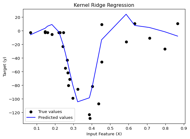
In problem which involves a distance between point, it is a common practice to normalize the data. In this notebook, we are going to normalize the data by dividing the time by 60 to convert it from minutes to hours (and have values between 0 and 1). We are going to use the KernelRidge class from the sklearn library to fit the KRR model. We will start by using the Gaussian/RBF kernel which is defined by: \[
K(x, x') = \exp\left(-\gamma||x - x'||^2\right)
\] where \(\gamma\) is an hyperparameter.
/Users/cherylkouadio/Documents/Repositories/website/venv/lib/python3.14/site-packages/tqdm/auto.py:21: TqdmWarning: IProgress not found. Please update jupyter and ipywidgets. See https://ipywidgets.readthedocs.io/en/stable/user_install.html
  from .autonotebook import tqdm as notebook_tqdm
# Load the datamcycle_data = pd.read_csv("Data/mcycle.csv")mcycle_data["times"] = mcycle_data["times"]/60mcycle_data.describe()
times
accel
count
133.000000
133.000000
mean
0.419649
-25.545865
std
0.218868
48.322050
min
0.040000
-134.000000
25%
0.260000
-54.900000
50%
0.390000
-13.300000
75%
0.580000
0.000000
max
0.960000
75.000000
# Split the data into train and test sampleX = mcycle_data[["times"]]y = mcycle_data[["accel"]]X_train, X_test, y_train, y_test = train_test_split(X, y, test_size=0.2, random_state=42)
1. Training and testing RBF kernel ridge regression
Since we have two hyperparameter (\(\gamma\) and \(\lambda\)) to tune, we can use the GridSearchCV function from scikit-learn to find the best hyperparameter.
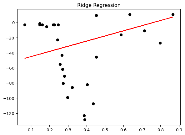
Now we are going to use the basic ridge regression to predict the target variable. There is only one hyperparameter to tune which is the regularization parameter \(\lambda\).
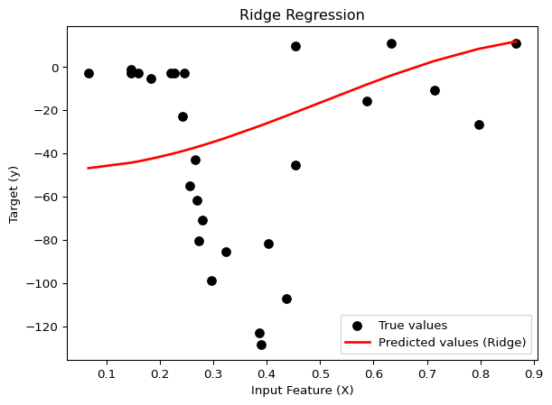
As we can see, the solelly use of the ridge regression is not enough to predict the target variable. We can try to transform the data by using a sinusoïdal transformation. If we try a transformation of the covariable \(x\) by \(\tilde{x}=\frac{\sqrt(2)}{\pi}\cos(\pi x)\) and apply the ridge regression, we have a slightly different problem. But still, the performance of the model is not good.
# create a function that apply transformation to the featuresdef apply_cos(x,j): pi = np.pireturn np.sqrt(2)*np.cos(j*pi*x)/(j*pi)# perform ridge regression with cosinus modification from j = 1 to 10X_train_cos = pd.DataFrame()X_test_cos = pd.DataFrame()for j inrange(1,11): X_train_cos[f"X{j}"] = X_train["times"].apply(lambda x: apply_cos(x,j)) X_test_cos[f"X{j}"] = X_test["times"].apply(lambda x: apply_cos(x,j))
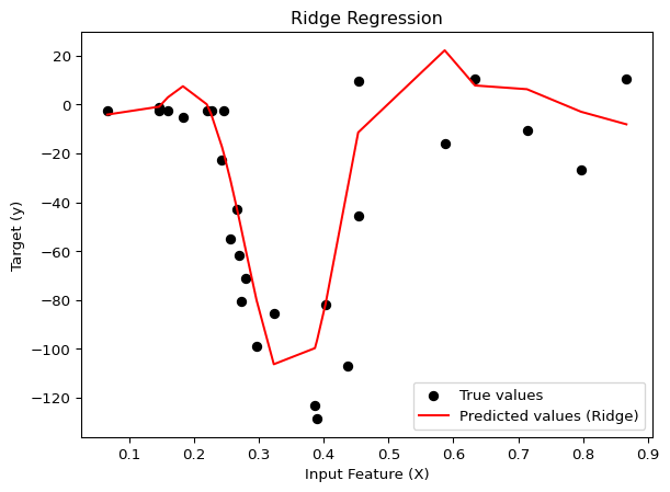
Even though, the only transformation applied is the cosinus transformation, the RMSE is lower than the RMSE of the simple Ridge Regression. This is due to the fact that the cosinus transformation is able to capture a little bit of the periodicity of the data. Let’s try to use many sinusoidal transformation to see if we can improve the performance of the model. We will fit y using \(\tilde{x} = \left[ \frac{\sqrt(2)}{J\pi}\cos(J\pi x) \right]_{J=1,\dots,10}\)
# New ridge with many transformated featuresridge_model2 = RidgeCV(alphas=grid_eval).fit(X_train_cos, y_train)y_pred_ridge2 = ridge_model2.predict(X_test_cos)y_pred_ridge2_sorted = y_pred_ridge2[sorted_indices]print( f'RMSE Ridge regression : {math.sqrt(mean_squared_error(y_test, y_pred_ridge2)): .2f}')# Plot the resultsplt.scatter(X_test, y_test, color="black",label="True values")plt.plot(X_test_sorted, y_pred_ridge2_sorted,color="red",label="Predicted values (Ridge)")plt.title("Ridge Regression")plt.xlabel("Input Feature (X)")plt.ylabel("Target (y)")plt.legend(loc="best")plt
RMSE Ridge regression : 22.96
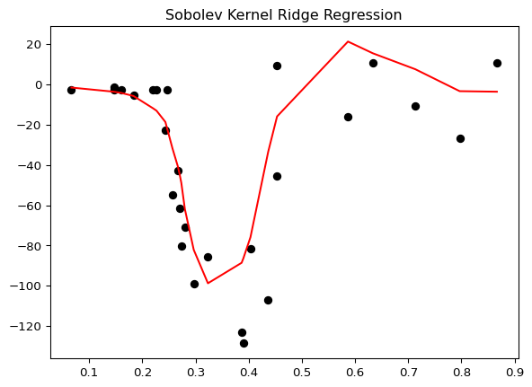
We observe that the more we increase the number of transformations, the more the performance of the model is improved and close to the performance of the kernel ridge regression using the gaussian kernel. The performance of the model is similar to the performance of the kernel ridge regression. This is due to the fact that the kernel ridge regression is equivalent to use an infinite number of transformations on the features. It is hence useful to use the kernel trick when we have a non-linear relationship between the target variable and the features.
III. Insigths :
Linear regression with such sinusoidal transformation is equivalent to the kernel ridge regression with a specific kernel : the sobolev kernel. The sobolev kernel is defined by: \[
K(x, x') = 1 + B_1(x)B_2(x') + \frac{1}{2}B_2(|x-x'|) = 1 + B_2(\frac{|x-x'|}{2}) + B_2(\frac{x+x'}{2})
\]
where \(B_1 = x - 1/2\) and \(B_2 = x^2 - x - 1/6\).
Using the fourier series expansion for \(x \in [0,1]\), we have : \[
B_2(x) = \sum_{k=1}^{\infty} \frac{\cos(2k\pi x)}{(k\pi)^2}
\]
Kernel de sobolev
def sobolev_kernel(x,y):def B2(x):return x**2- x +1/6def B1(x):return x -1/2return1+ B2(abs(x-y)/2) + B2((x+y)/2)
The support vector machines (SVM) is a supervised learning algorithm that can be used for classification. The SVM is based on the concept of finding the hyperplane that best separates the data into two classes. In fact, if the problem is linearly separable, the SVM finds the hyperplane that maximizes the margin between the two classes. The margin is the distance between the hyperplane and the closest point of each class (support vectors).
When the problem is non-linearly separable, the SVM uses the same functionnement but allows some points to be misclassified. When the problem is too complex, the SVM uses the kernel trick to transform the data into a higher-dimensional space where the relationship is linear.
I. Toy dataset
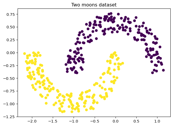
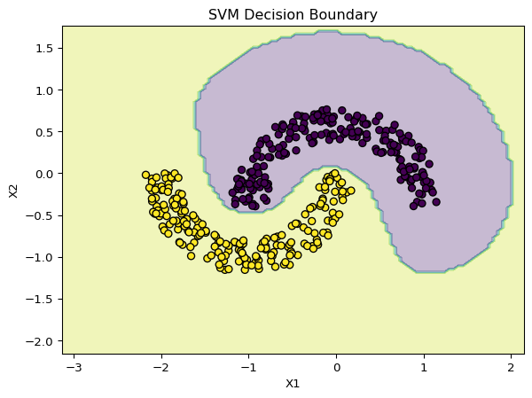
Here is the toy dataset that we are going to use to illustrate the SVM. The dataset is composed of two features and the target variable is binary. As we can see, the dataset is not linearly separable. We are going to use the SVM with a gaussian kernel to classify the data, and compare it to a classic classifier such as the k-nearest neighbors and the logistic regression.
# Split the data into train and test sampleX_train, X_test, y_train, y_test = train_test_split(two_moon_data[["X1","X2"]], two_moon_data["y"], test_size=0.2, random_state=42)
1. K-nearest neighbors
# KNN with cross validationknn = KNeighborsClassifier()param_grid = {"n_neighbors": np.arange(1, 50)}knn_cv = GridSearchCV(knn, param_grid).fit(X_train, y_train)print(f"Best parameters by CV : {knn_cv.best_params_}")# Compute the accuracyy_pred = knn_cv.predict(X_test)accuracy = accuracy_score(y_test, y_pred)print(f"Accuracy: {accuracy:.2f}")# Confusion matrix to see detailed classification performanceconf_matrix = confusion_matrix(y_test, y_pred)print("Confusion Matrix:")print(conf_matrix)# Classification report for detailed metricsprint("Classification Report:")print(classification_report(y_test, y_pred))
As we can see, the SVM with the gaussian kernel is able to classify the data with a good accuracy. The SVM is able to capture the non-linear relationship between the target variable and the features.
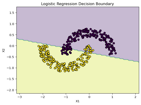
The logistic regression, in this case, is not able to classify the data because the relationship between the target variable and the features is non-linear.
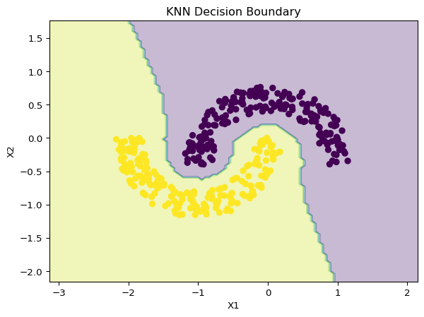
The k-nearest neighbors is able to classify the data with a performance similar to the SVM. The SVM and the KNN are a good choice when we have a non-linear relationship between the target variable and the features.
Whenever we have a classification problem, it is hence always useful to try the SVM and the KNN.
II. Image dataset
The SVM is also useful for image classification. In this part, we are going to use the famous MNIST dataset to classify the images. The MNIST dataset is composed of 20 000 images (10 000 in the training dataset, and 10 000 also in the test dataset) of handwritten digits from 0 to 9. Each image is a resolution 28x28 pixels that is represented by a matrix of shape (28, 28), with each element being the pixel intensity (values from 0 to 255). We are going to use the SVM with the gaussian kernel to classify the images.
We will start by normalizing the data to ensure that all the features contribute equally, and then use the GridSearchCV function from scikit-learn to find the best hyperparameter.
data_train = pd.read_csv("Data/mnist_train_small.csv")data_test = pd.read_csv("Data/mnist_test.csv")print("Description of train dataset : \n")data_train.iloc[:,1:].describe()data_train["label"].value_counts()
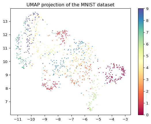
As we can see from the umap plot, which is a dimensionality reduction technique, the data is not always linearly separable. We are going to use the SVM with the gaussian kernel to classify the images.
# visualize the data with UMAPreducer = umap.UMAP(random_state=42)embedding = reducer.fit_transform(X_train)
plt.scatter(embedding[:, 0], embedding[:, 1], c=data_train["label"], cmap='Spectral', s=1)plt.gca().set_aspect('equal', 'datalim')plt.colorbar()plt.title('UMAP projection of the MNIST dataset')
Text(0.5, 1.0, 'UMAP projection of the MNIST dataset')
svm_model = SVC(kernel="rbf")from itertools import productgrid_eval_C = [c * factor for c, factor in product([0.1, 1, 10], [1, 5])]grid_eval_gamma = [gamma * factor for gamma, factor in product([10**-3, 10**-2, 10**-1], [1, 5])]param_grid = {"C": grid_eval_C, "gamma": grid_eval_gamma}svm_model_cv = GridSearchCV(svm_model, param_grid).fit(X_train, y_train)print(f"Best parameters by CV : {svm_model_cv.best_params_}")
Best parameters by CV : {'C': 5, 'gamma': 0.001}
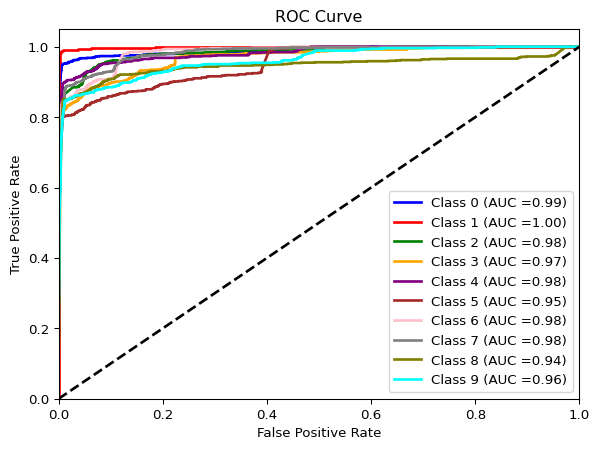
As we can see, the model performs well with an accuracy of 0.88 . As expected from the umap visualization, the model is able to separate the classes well, however there are some errors in the classification. The confusion matrix shows that the model has some difficulty to distinguish between some digits such as 4 and 9, 3.
The SVM is a good choice for image classification, however, the model is not able to capture the complexity of the data. In this case, we can use a deep learning model such as the convolutional neural network (CNN) which is able to capture the complexity of the data.
# compute the accuracyy_pred = svm_model_cv.predict(X_test)accuracy = accuracy_score(y_test, y_pred)print(f"Accuracy: {accuracy:.2f}")# Confusion matrix to see detailed classification performanceconf_matrix = confusion_matrix(y_test, y_pred)print("Confusion Matrix:")print(conf_matrix)# Classification report for detailed metricsprint("Classification Report:")print(classification_report(y_test, y_pred))